A little mini-meme got started on August 1 when
Ben Bolker
posted the following code
to the
r-devel list (and here I substituted the more standard '-' assignment
operator for the less standard though-now permitted '='):
x <- readLines("http://developer.r-project.org/R.svnlog.2007")
rx <- x[grep("^r",x)]
who <- gsub(" ","",sapply(strsplit(rx,"\\ "),"[",2))
twho <- table(who)
twho["ripley"]/sum(twho)
In five lines (that could be shortened to three at the expense of some
readibility), the SVN log for
R is
downloaded directly from the website, the revision authors are extraced and then
tabulated by submitter. The relative percentage of Brian Ripley is found
to be a staggering 74.8% -- or about three times as much as the other fifteen
committers combined. Smokes.
[ Oh, and for those who don't know him, he's also got a day job which presumably
entails looking after his graduate students at Oxford. Who knows, he may even
teach. Kidding aside, he's actually one of the nicest persons you'll ever
meet in real life. ]
Now yesterday,
Simon Jackman who
had at first simply repeated Ben's analysis on his own
blog followed up with a nice
analysis (albeit typeset in a way that rendered the code inoperational, which
has now been fixes) that creates both a histogram and a dotplot of commits
per hour of the day. Omitting Ben's code which Simon reuses, we have the
following for histogram and dotchart:
tod <- unlist(sapply(rx,function(x)strsplit(x,split=" ")[[1]][6]))
tod <- tod[who=="ripley"]
tz <- sub(pattern=".*(-[0-9] 4 ).*",replacement="\\1",x=rx)
tz <- tz[who=="ripley"]
tz <- as.numeric(tz)/100
offset <- 3600*tz
z <- strptime(tod,format="%H:%M:%S")
hist(z,"hours",main="Ripley Commit Times in SVN TZ")
h <- z - offset
h <- format(h,format="%H")
h <- factor(as.numeric(h), levels=0:23)
dotchart(table(h), main="Ripley Commit Times, By Hour in GMT",
         labels=paste(0:23,1:24,sep=":"))
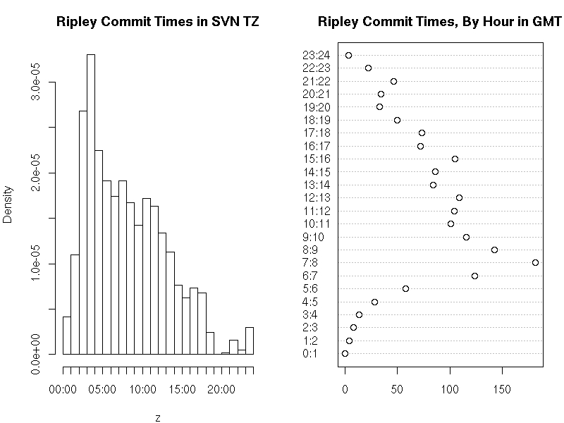
This extracts the commit times, subsets to the ones by Prof. Ripley, extracts
the timezones component (as
strptime seemingly doesn't do that
which is a pain), extracts the tz-less time via
strptime into a
variable 'z' for which the histogram is drawn. He then corrects the times by
the tz offset expressed in seconds, formats is as hour of the day and turns
it into a 'factor' (an R data type for qualitative variables which may be
ordered as is the case here) and draws a dotplot. This results in the
following chart:
Now, nobody has looked at the time series. So we correct this and add the
following:
## rather extract both  date and time
dat <- unlist(sapply(rx, function(x)
  txt <- strsplit(x,split=" ")[[1]]
  paste(txt[5], txt[6])
 ))
## subset on Prof Ripley
dat <- dat[who == "ripley"]
## and convert to POSIXct, correcting by tz as well
datpt <- as.POSIXct(strptime(dat,format="%Y-%m-%d %H:%M:%S")) - offset
## turn into zoo -- we use a constant series of ones as each
## committ is taken as a timestamped event
datzoo <- zoo(1, order.by=datpt)
## and use zoo to aggregate into commits per date
daily <- aggregate(datzoo, as.Date(index(datzoo)), sum)
## now plot as grey bars
plot(daily, col='darkgrey', type='h', lwd=2,
     ylab="Nb of SVN commits, three-week median",
     xlab="R release dates 2.5.0 and 2.5.1 shown in orange",
     main="The amazing Prof. Ripley")
## mark the two R releases of 2007
abline(v=c(as.Date("2007-04-24"),as.Date("2007-06-28")),col='orange',lwd=1.5)
## and do a quick centered rolling median
lines(rollmedian(daily, 21, align="center"), lwd=3)
This extracts both date and time, creates a proper R time object (a so-called
POSIXct type) from it, fills a zoo ('the' magic class for time series) object
with it, uses zoo to aggregate commits per day and plots those in a
barchart-alike (I know, I know, ...) plot to which we add the two releases as
well as a rolling and centered three-week median (as a real quick hack rather
than a proper smooth).
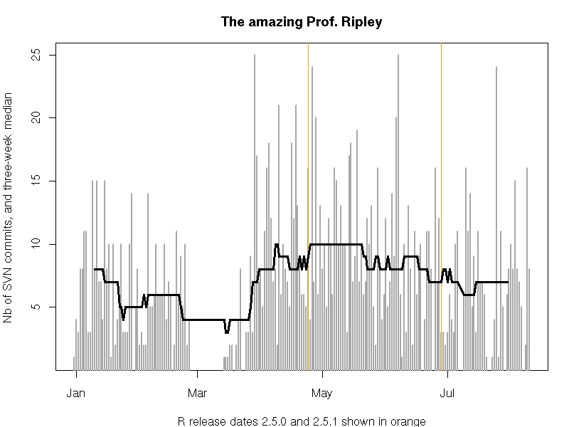
This shows that Prof Ripley averaged about ten
commits a day before and after the release of R 2.5.0, and that he has slowed
down ever so slightly since then to end up at around a mere seven commits a
day. Every day. For the seven-plus months we looked at.
So, anyone for analysing his r-help posting frequencies ?


 In case you got one of those “Telekom Speedport 200” AKA “Tecom Tiny
Bridge DSL Modem” too you may want to fetch the script and have fun.
Just link it into the munin plugins dir as dsl_[rate snr attenuation]
and restart munin-node. A few mins later graphs should appear.
In case you improve it (its a quick hack only) I would love to get some
patches. :)

